Beyond pairwise correlation: capturing nonlinear and higher-order dependence with distance statistics

Motivating examples

This section provide the codes for generating the figures and statistics in the introduction of the paper, as well as the data generation process for simulated data.

2020 birth and death rates

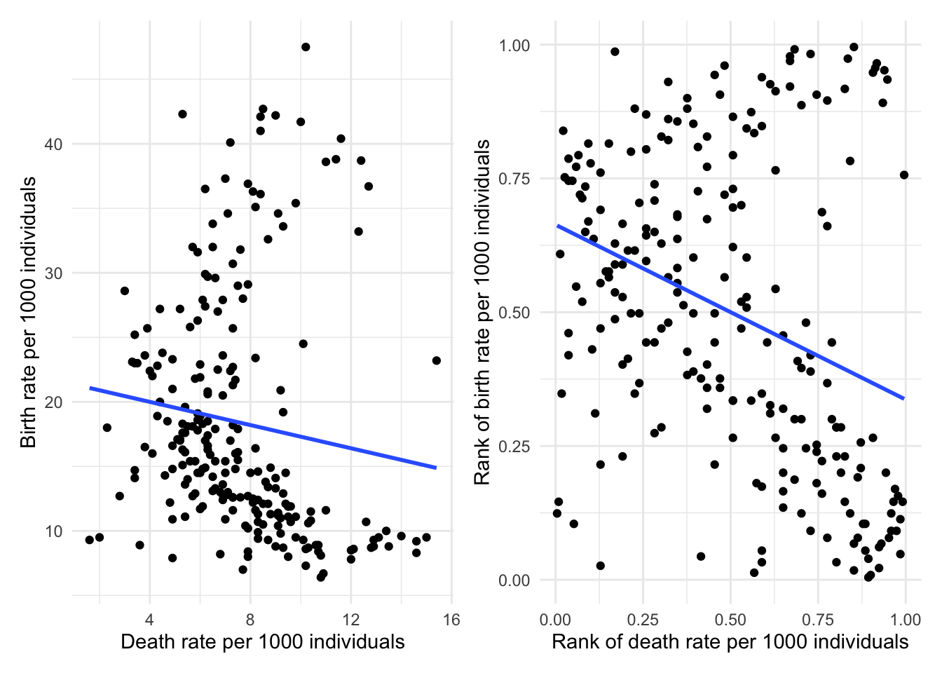
Our first motivating example involves the birth and death rate data from different countries in the first trimester of 2020 (Central Intelligence Agency 2020). This example is to illustrate that correlations are inherently for linear and monotonic relationships and hence a 0 correlation does not mean independence, and a small value does not necessarily means the actual dependence relationship is weak.

The birth and death rates are measured as the numbers of births and deaths per 1000 individuals, respectively, across 229 countries. The data can be loaded through the HellCor package in R.

Figure 2.1

# Load birth vs death rate data
data("worlddemographics")

# Transform the data into ranks
worlddemographics_rank <- worlddemographics |>
  transform(
    FDeath = rank(Death.Rate.Pop) / (nrow(worlddemographics) + 1),
    FBirth = rank(Birth.Rate.Pop) / (nrow(worlddemographics) + 1)
  )

# Plotting both the raw data (p1) and the ranks (p2) out
p1 <- ggplot(worlddemographics, aes(x = Death.Rate.Pop, y = Birth.Rate.Pop)) +
  geom_point() +
  geom_smooth(method = "lm", se = FALSE) +
  labs(
    x = "Death rate per 1000 individuals",
    y = "Birth rate per 1000 individuals"
  ) +
  theme_minimal()

p2 <- ggplot(worlddemographics_rank, aes(x = FDeath, y = FBirth)) +
  geom_point() +
  geom_smooth(method = "lm", se = FALSE) +
  labs(
    x = "Rank of death rate per 1000 individuals",
    y = "Rank of birth rate per 1000 individuals"
  ) +
  theme_minimal()

p1 + p2

`geom_smooth()` using formula = 'y ~ x'
`geom_smooth()` using formula = 'y ~ x'

The corresponding correlation coefficients, and the corresponding \(p\)-values with the null hypothesis \[ \begin{aligned} H_0 &: \theta=0,\\ H_1 &: \theta\neq0, \end{aligned} \] for \(\theta\in\{r \text{ (Pearson)}, \rho \text{ (Spearman)}, \tau \text{ (Kendall)}\}\) are given by

# Getting raw data for birth and death
birth_raw <- worlddemographics$Birth.Rate.Pop
death_raw <- worlddemographics$Death.Rate.Pop

set.seed(123) # This is for bootstrap test for correlation
cor_matrix_birth_death <- rbind(
  correlation = c(
    cor.test(birth_raw, death_raw, method = "pearson")$estimate,
    cor.test(birth_raw, death_raw, method = "spearman")$estimate,
    cor.test(birth_raw, death_raw, method = "kendall")$estimate
  ),
  p_value = c(
    # p-val for Pearson's corr needs boostrap here
    # As the null of the t-test assumed bivariate normal,
    # which is not necessarily true in this case.
    TOSTER::boot_cor_test(birth_raw, death_raw)$p.value, 
    cor.test(birth_raw, death_raw, method = "spearman")$p.value,
    cor.test(birth_raw, death_raw, method = "kendall")$p.value
  )
)

colnames(cor_matrix_birth_death) <- c("Pearson", "Spearman", "Kendall")
cor_matrix_birth_death

                Pearson      Spearman       Kendall
correlation -0.12513158 -3.268202e-01 -2.359474e-01
p_value      0.06503252  4.232096e-07  1.319531e-07

Multi-line example

The other example is used to illustrate that the correlation is inherently pairwise, and it cannot detect association when the underlying association exist when they considered jointly. For this example, there are two business lines where we have the motor line with the following components: \[\begin{equation*} \mathbf{X}=(X_1,X_2,X_3)=\text{(vehicle repair cost, bodily injury liability, claims handling cost)}, \end{equation*}\] and \(Y\) denotes the medical claim cost recorded under another line of business. The data is simulated using the following code

set.seed(123)
n <- 5000

U1 <- runif(n) # latent for vehicle repair
U2 <- runif(n) # latent for bodily injury liability
U3 <- runif(n) # latent for claims handling

# latent for medical claims - it depends on both 
# vehicle damage and bodily injury
C <- (U1 + U2) %% 1 

# Independently distributed in Gamma
X1 <- qgamma(U1, shape = 2.5, scale = 2000)
X2 <- qgamma(U2, shape = 3.0, scale = 3000)

# Gamma as well, but dependends on (X1, X2)
Y <- qgamma(C, shape = 2.2, scale = 2500)

# Here we have claims handling cost, and there are two types of claim:
# Severity driven: handling cost goes up with medical cost (C)
# Review driven: handling cost higher for smaller medical cost (1-C)
p <- 0.50
R <- rbinom(n, size = 1, prob = p)
W <- ifelse(R == 1, C, 1 - C)

X3 <- qgamma(W, shape = 2.0, scale = 1200)

multi_line_dat <- data.frame(X1,X2,X3,Y)

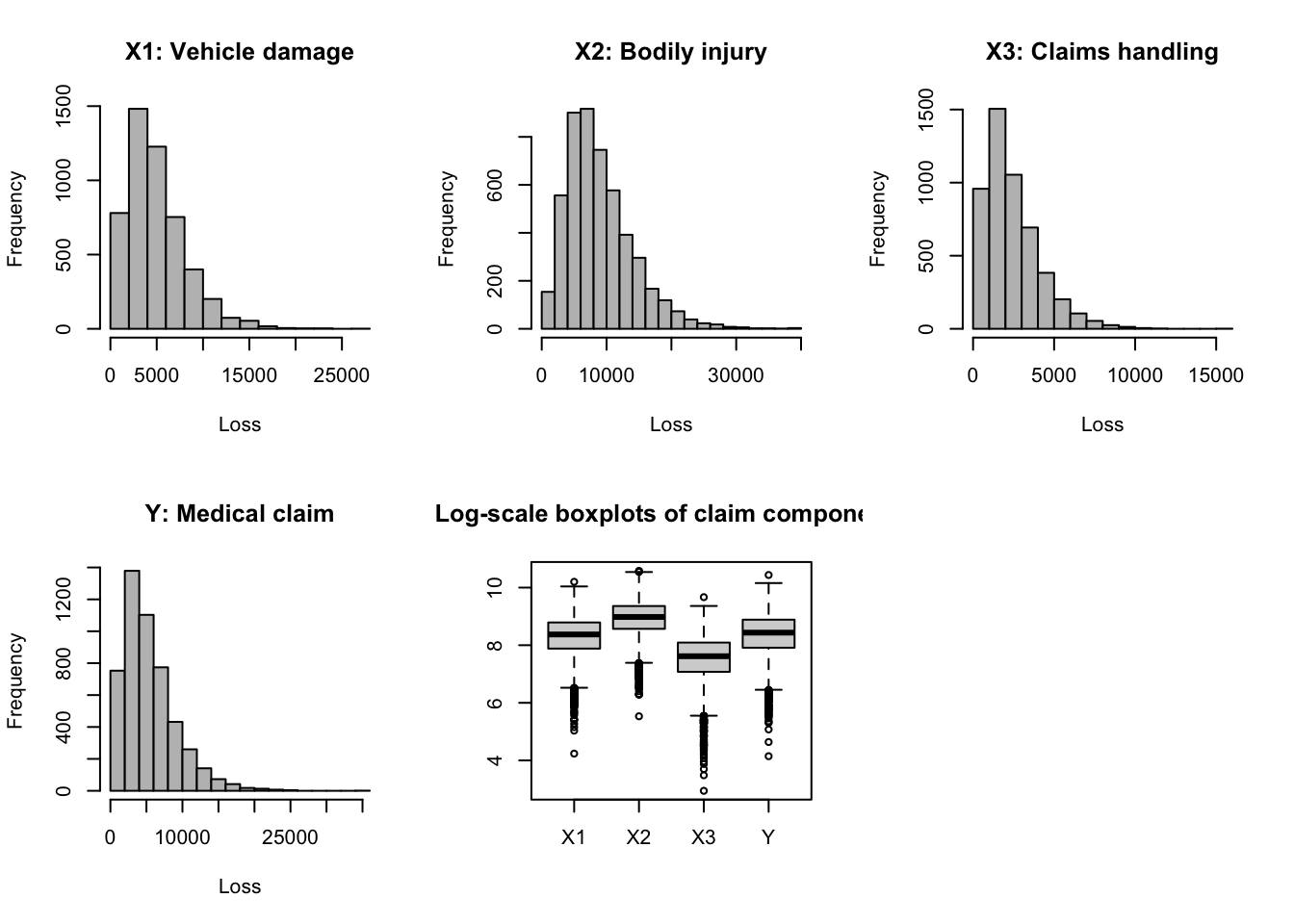
Below we apply some exploratory data analysis. First, we look at the distribution of each of the claim costs. As expected, all of the shape looks like a \(\Gamma\)-distribution:

Figure 2.2

par(mfrow = c(2,3))

# Histogram for each of the claim costs
hist(multi_line_dat$X1, main = "X1: Vehicle damage", xlab = "Loss", col = "grey")
hist(multi_line_dat$X2, main = "X2: Bodily injury", xlab = "Loss", col = "grey")
hist(multi_line_dat$X3, main = "X3: Claims handling", xlab = "Loss", col = "grey")
hist(multi_line_dat$Y, main = "Y: Medical claim", xlab = "Loss", col = "grey")

# Boxplot for log claim components
boxplot(log(multi_line_dat[, c("X1","X2","X3","Y")]),
        main = "Log-scale boxplots of claim components")

Then, we apply bivariate analysis. First, we plot the scatter plots for each pair of the variables using their ranks. Here ranks are used to reveal the dependence structure between the pairs.

Figure 2.3

# plot the scatterplots on the ranks for each claim variable
Fx1 <- ecdf(multi_line_dat$X1)(multi_line_dat$X1)
Fx2 <- ecdf(multi_line_dat$X2)(multi_line_dat$X2)
Fx3 <- ecdf(multi_line_dat$X3)(multi_line_dat$X3)
Fy  <- ecdf(multi_line_dat$Y)(multi_line_dat$Y)

png("cross_pair_multiline_rank.png", width = 4800, height = 3200, res = 600)

par(mfrow = c(2,2))
plot(Fx1, Fy, pch = 16, cex = 0.35,
     xlab = "Empirical CDF of X1", ylab = "Empirical CDF of Y",
     main = "Medical claim (Y) vs vehicle damage (X1)")

plot(Fx2, Fy, pch = 16, cex = 0.35,
     xlab = "Empirical CDF of X2", ylab = "Empirical CDF of Y",
     main = "Medical claim (Y) vs bodily injury (X2)")

plot(Fx2, Fx1, pch = 16, cex = 0.35,
     xlab = "Empirical CDF of X2", ylab = "Empirical CDF of X1",
     main = "Vehicle damage (X1) vs bodily injury (X2)")

plot(Fx3, Fy, pch = 16, cex = 0.35,
     xlab = "Empirical CDF of X3", ylab = "Empirical CDF of Y",
     main = "Medical claim (Y) vs claims handling (X3)")
dev.off()

quartz_off_screen 
                2 

The correlation and the corresponding \(p\)-value matrices are given by below:

get_pmat_corr <- function(dat, method = c("pearson", "spearman", "kendall"),
                          R = 9999) {
  # This function is used to get the p-values for testing correlation significance
  # Input: a dataframe with all numerical columns
  # output: p-value matrix of the choice of correlation
  method <- match.arg(method)
  
  dat <- as.data.frame(dat)
  pmat <- matrix(NA_real_, ncol(dat), ncol(dat))
  colnames(pmat) <- rownames(pmat) <- colnames(dat)
  
  for (i in 1:(ncol(dat) - 1)) {
    for (j in (i + 1):ncol(dat)) {
      x <- dat[[i]]
      y <- dat[[j]]
      
      keep <- complete.cases(x, y)
      x <- x[keep]
      y <- y[keep]
      
      pval <- if (method == "pearson") {
        TOSTER::boot_cor_test(x, y, method = "pearson", null = 0, alternative = "two.sided", R = R)$p.value
      } else {
        cor.test(x, y, method = method)$p.value
      }
      
      pmat[i, j] <- pval
      pmat[j, i] <- pval
    }
  }
  
  diag(pmat) <- NA
  pmat
}

cor(multi_line_dat) # Pearson correlation

             X1           X2          X3           Y
X1  1.000000000 -0.025932480 0.001279202 -0.01000060
X2 -0.025932480  1.000000000 0.006776664 -0.02001201
X3  0.001279202  0.006776664 1.000000000  0.07614912
Y  -0.010000596 -0.020012013 0.076149119  1.00000000

get_pmat_corr(multi_line_dat, method = "pearson")

          X1        X2        X3         Y
X1        NA 0.0870087 0.9362936 0.4866487
X2 0.0870087        NA 0.6576658 0.1978198
X3 0.9362936 0.6576658        NA 0.0050005
Y  0.4866487 0.1978198 0.0050005        NA

cor(multi_line_dat, method = "spearman") # Spearman correlation

             X1           X2           X3           Y
X1  1.000000000 -0.019885108 -0.009221736 -0.01336648
X2 -0.019885108  1.000000000  0.007085466 -0.02314468
X3 -0.009221736  0.007085466  1.000000000 -0.01399048
Y  -0.013366483 -0.023144684 -0.013990480  1.00000000

get_pmat_corr(multi_line_dat, method = "spearman")

          X1        X2        X3         Y
X1        NA 0.1597607 0.5144489 0.3446798
X2 0.1597607        NA 0.6164421 0.1017588
X3 0.5144489 0.6164421        NA 0.3226253
Y  0.3446798 0.1017588 0.3226253        NA

cor(multi_line_dat, method = "kendall") # Kendall correlation

             X1           X2           X3            Y
X1  1.000000000 -0.013227766 -0.006103941 -0.008739668
X2 -0.013227766  1.000000000  0.004754391 -0.015579916
X3 -0.006103941  0.004754391  1.000000000 -0.012888658
Y  -0.008739668 -0.015579916 -0.012888658  1.000000000

get_pmat_corr(multi_line_dat, method = "kendall")

          X1         X2        X3          Y
X1        NA 0.16075838 0.5175063 0.35410443
X2 0.1607584         NA 0.6141891 0.09855056
X3 0.5175063 0.61418909        NA 0.17176004
Y  0.3541044 0.09855056 0.1717600         NA

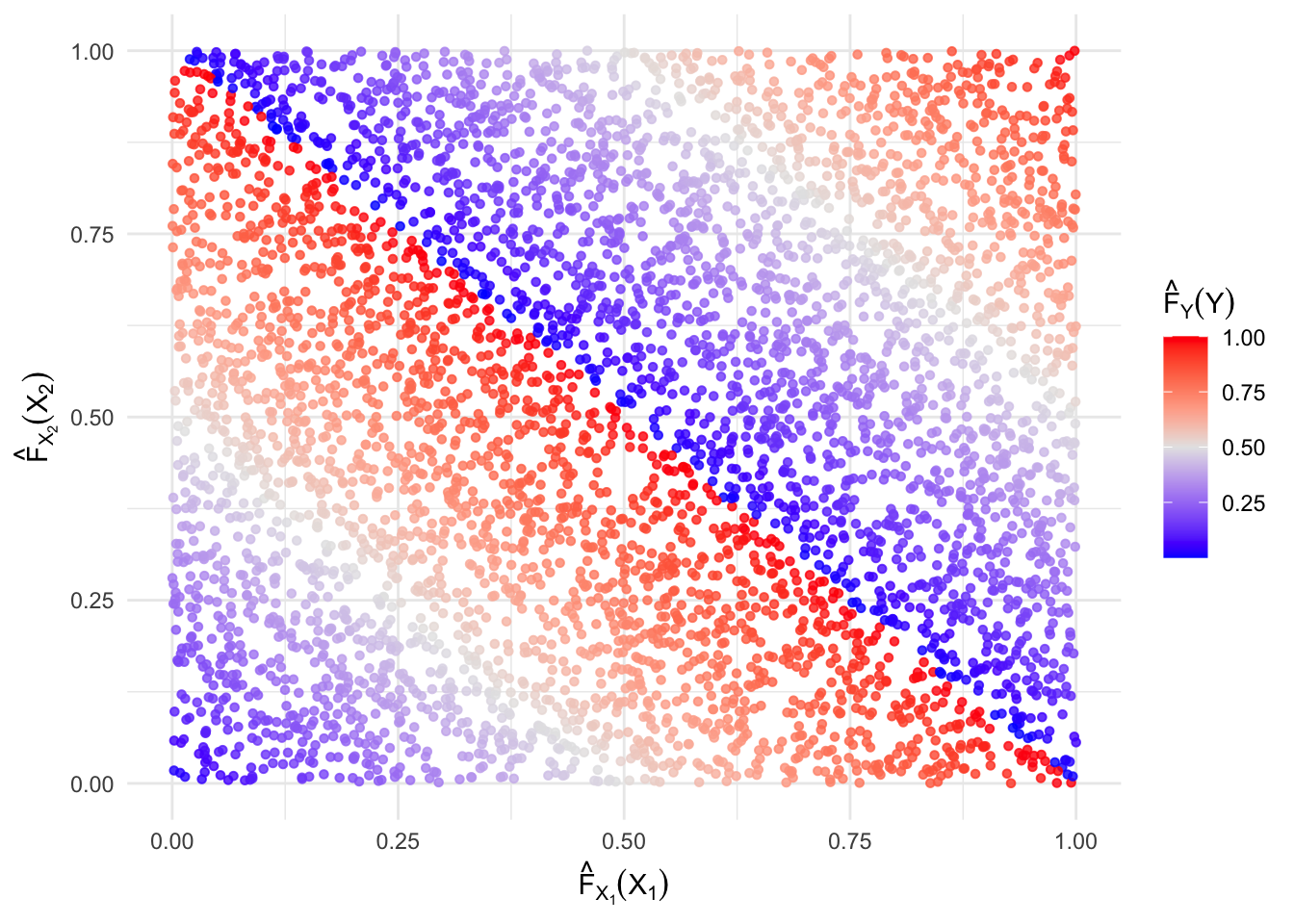
Here, as we can see the pairs \((X_1,X_2)\), \((X_1,Y)\), and \((X_2,Y)\) does not show any obvious pattern, suggesting independence. However, when we look at the scatter plot between \((X_1,X_2)\) coloured by \(Y\), we can see that the value of \(Y\) forms a diganoal pattern, i.e. knowing the value of \((X_1,X_2)\) provide information of \(Y\), suggesting that they are not mutually independent. This raise one of the pitfall that correlation, and in general, thinking in pairwise dependence, can miss strutures where the dependence is considered jointly.

Figure 2.4(a)

# build eCDF for the multi-line data
multi_line_ECDF <- multi_line_dat %>%
  mutate(
    FX1 = rank(X1) / n(),
    FX2 = rank(X2) / n(),
    FX3 = rank(X3) / n(),
    FY = rank(Y) / n()
  )

ggplot(multi_line_ECDF, aes(x = FX1, y = FX2, colour = FY)) + 
  geom_point(size = 1.2, alpha = 0.8) + 
  scale_colour_gradient2(
    low = "blue",
    mid = "grey90",
    high = "red",
    midpoint = 0.5,
    name = expression(hat(F)[Y](Y))
  ) +
  labs(
    x = expression(hat(F)[X[1]](X[1])),
    y = expression(hat(F)[X[2]](X[2]))
  ) + 
  theme_minimal()

Figure 2.4(b)

# get pseudo-observations of the data (i.e. eCDF)
pseudo_obs <- function(x) {
  rank(x, ties.method = "average", na.last = "keep") / (sum(!is.na(x)) + 1)
}

# Map concentration of points to [0,1]
# 0 = blue, 0.5 = white, 1 = red
mid_rescale <- function(x, low, mid, high) {
  out <- numeric(length(x))

  left  <- x <= mid
  right <- x > mid

  out[left]  <- 0.5 * (x[left]  - low) / (mid - low)
  out[right] <- 0.5 + 0.5 * (x[right] - mid) / (high - mid)

  out[!is.finite(out)] <- 0.5
  pmin(pmax(out, 0), 1)
}

# compute the concentration at each point
build_concentration_scores <- function(dat,
                                       x_col = "X1",
                                       y_col = "X2",
                                       z_col = "Y",
                                       r = NULL,
                                       scale = c("absolute", "relative")) {
  scale <- match.arg(scale)

  df <- dat %>%
    dplyr::select(all_of(c(x_col, y_col, z_col))) %>%
    na.omit()

  names(df) <- c("x", "y", "z")

  U <- df %>%
    dplyr::mutate(
      u1 = pseudo_obs(x),
      u2 = pseudo_obs(y),
      u3 = pseudo_obs(z)
    )

  Umat <- as.matrix(U[, c("u1", "u2", "u3")])
  n <- nrow(Umat)

  if (is.null(r)) {
    r <- 0.61 * n^(-0.18)
  }

  # pairwise Euclidean distances in pseudo-observation space
  D <- as.matrix(dist(Umat))
  diag(D) <- NA_real_

  # Step 1: raw local mass inside radius r
  h_raw <- rowMeans(D <= r, na.rm = TRUE)

  # Step 2: inverse-distance weighted smoothing
  h_hat <- vapply(seq_len(n), function(i) {
    nbr <- which(D[i, ] <= r)

    if (length(nbr) == 0) {
      return(h_raw[i])
    }

    d <- D[i, nbr]
    d[d == 0] <- min(d[d > 0], na.rm = TRUE)
    if (!any(is.finite(d))) {
      return(h_raw[i])
    }

    w <- 1 / d
    sum(w * h_raw[nbr]) / sum(w)
  }, numeric(1))

  # independence benchmark for a 3D ball
  h0 <- 4 * pi * r^3 / 3

  if (scale == "absolute") {
    low  <- 0
    high <- 2 * r / sqrt(3)
  } else {
    low  <- min(h_hat)
    high <- max(h_hat)
    if (low == high) {
      low  <- low - 1e-8
      high <- high + 1e-8
    }
  }

  score <- mid_rescale(h_hat, low = low, mid = h0, high = high)

  U %>%
    mutate(
      h_raw = h_raw,
      h_hat = h_hat,
      colour_score = score,
      radius = r
    )
}

# 3D plot: U1, U2, Y
plot_3d <- function(scored_df) {
  plot_ly(
    data = scored_df,
    x = ~u1, y = ~u2, z = ~u3,
    type = "scatter3d",
    mode = "markers",
    marker = list(
      size = 3,
      color = ~colour_score,
      cmin = 0,
      cmax = 1,
      colorscale = list(
        c(0.0, "blue"),
        c(0.5, "whitesmoke"),
        c(1.0, "red")
      ),
      showscale = TRUE,
      colorbar = list(title = "Concentration")
    )
  ) %>%
    layout(
      scene = list(
        xaxis = list(title = list(text = "F<sub>X1</sub>(X1)")),
        yaxis = list(title = list(text = "F<sub>X2</sub>(X2)")),
        zaxis = list(title = list(text = "F<sub>Y</sub>(Y)"))
      )
    )
}

# run code on multi-line data
scores_X1X2Y <- build_concentration_scores(
  dat   = multi_line_dat,
  x_col = "X1",
  y_col = "X2",
  z_col = "Y",
  scale = "absolute"
)

plot_3d(scores_X1X2Y)

Failure of CLT

Another important implication of relying on pairwise dependence statistics is that, many of the actuarial modelling assumption relies on the assumption that the random variables are (mutually) independent and identically distributed. It is possible to construct a sequence of identical and pairwise independent random variables but not mutually independent. However, this cannot be detected through bivariate dependence statistics such as the correlation. And it is possible that the central limit theorem (CLT) fails for such a sequence of random variables.

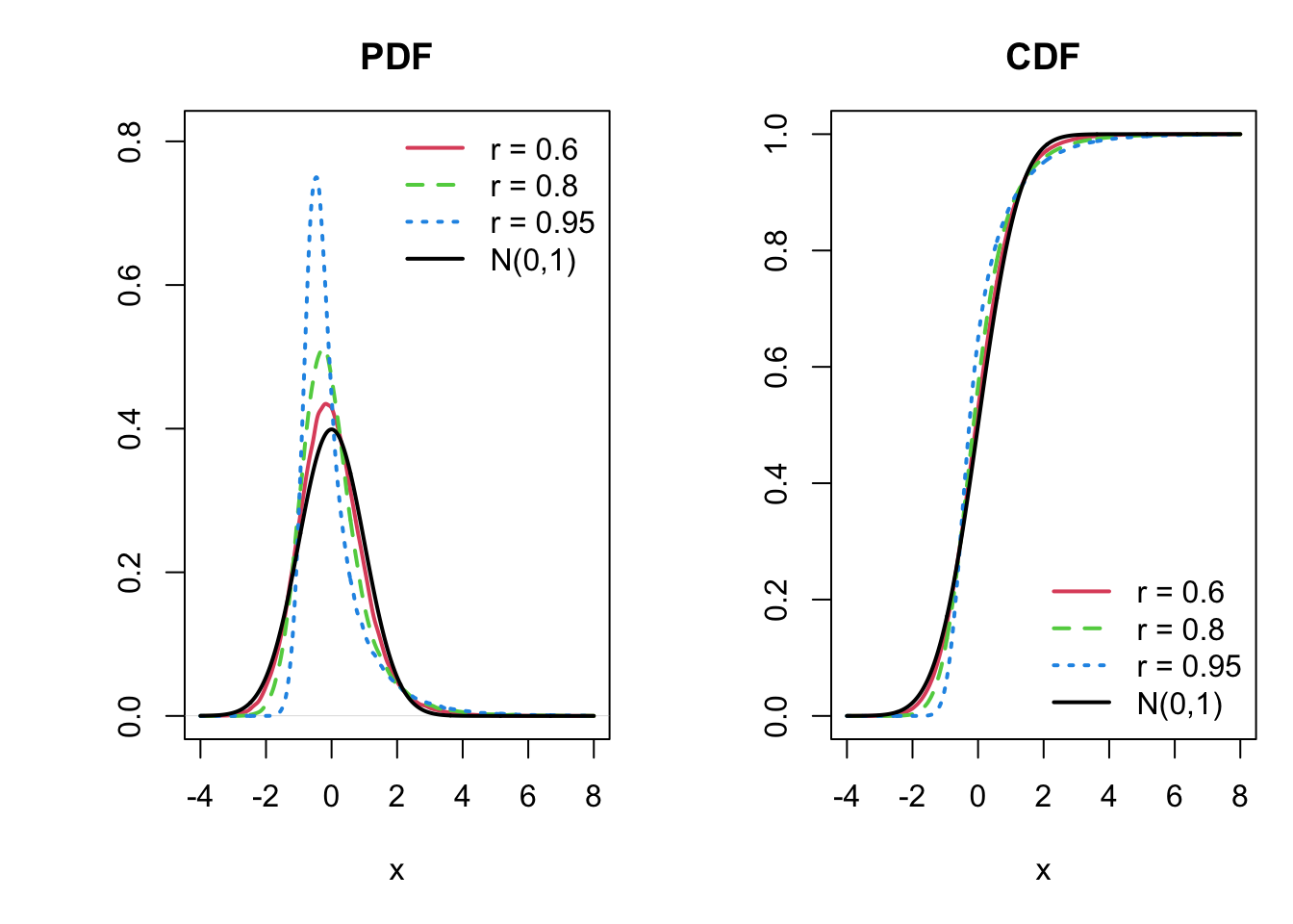
As illustrated by Avanzi et al. (2021) and Beaulieu et al. (2021), pairwise independence alone does not guarantee asymptotic normality. They construct a sequence \(X_1,\ldots,X_n\) of pairwise independent, but not mutually independent, standard normal random variables such that the limiting distribution of \[\begin{equation} \sqrt{n}\,\frac{1}{n}\sum_{i=1}^n X_i \end{equation}\] coincides with that of the random variable \[\begin{equation}\label{eq:limit_dist} S=\sqrt{1-r^2}\,Z+r\chi, \end{equation}\] where \(Z\sim N(0,1)\), \(\chi\) is a standardised chi-squared random variable independent of \(Z\), and \(0<r^2<1\). The limiting distribution does not necessarily converge to the normal distribution, as the CLT suggests.

Figure 2.5

set.seed(123)

# standardised chi-squared distribution with df = 1
rchi_std <- function(n){
  (rchisq(n, df = 1)-1)/sqrt(2)
}

# Limiting distribution
rS <- function(n, r){
  sqrt(1 - r^2) * rnorm(n) + r * rchi_std(n)
}

r_vals <- c(0.6, 0.8, 0.95)
n <- 300000
x_grid <- seq(-4, 8, length.out = 1000)

samples <- lapply(r_vals, function(r) rS(n, r))
densities <- lapply(samples, density,
                    from = min(x_grid), to = max(x_grid),
                    n = 1000)

ymax <- max(
  sapply(densities, function(d) max(d$y)),
  max(dnorm(x_grid))
)
ymax <- 1.08 * ymax

par(mfrow = c(1,2), mar = c(5,5,3,1))

# plot PDF 
plot(densities[[1]], type = "l", lwd = 2, col = 2,
     main = "PDF", xlab = "x", ylab = "",
     xlim = range(x_grid), ylim = c(0, ymax))

for (i in 2:length(densities)) {
  lines(densities[[i]], lwd = 2, col = i + 1, lty = i)
}
lines(x_grid, dnorm(x_grid), lwd = 2, col = 1)

legend("topright",
       legend = c(paste0("r = ", r_vals), "N(0,1)"),
       col = c(2, 3, 4, 1),
       lty = c(1, 2, 3, 1),
       lwd = 2,
       bty = "n")

# plot CDF 
plot(x_grid, ecdf(samples[[1]])(x_grid), type = "l", lwd = 2, col = 2,
     main = "CDF", xlab = "x", ylab = "",
     xlim = range(x_grid), ylim = c(0, 1))

for (i in 2:length(samples)) {
  lines(x_grid, ecdf(samples[[i]])(x_grid),
        lwd = 2, col = i + 1, lty = i)
}
lines(x_grid, pnorm(x_grid), lwd = 2, col = 1)

legend("bottomright",
       legend = c(paste0("r = ", r_vals), "N(0,1)"),
       col = c(2, 3, 4, 1),
       lty = c(1, 2, 3, 1),
       lwd = 2,
       bty = "n")

Illustrations

Now in this section we illustrate how the distance-based dependence statistics can be computed through R.

Illustrations using Hellinger correlation

library(HellCor) # this library is used to compute the Hellinger correlation

The first distance-based dependence statistic introduced is called the Hellinger correlation. Intuitively it measures the difference between the copula density between the two (continuous univariate) variables and the independence copula density.

Figure 3.1

n <- 55
eps <- 0.02
u <- seq(eps, 1 - eps, length.out = n)
v <- seq(eps, 1 - eps, length.out = n)
grid <- expand.grid(u = u, v = v)

# Independence density
z_indep <- matrix(1, nrow = n, ncol = n)

# Clayton copula density
theta <- 5
cop_clayton <- claytonCopula(param = theta, dim = 2)
z_clayton <- matrix(
  dCopula(as.matrix(grid), copula = cop_clayton),
  nrow = n, ncol = n
)
z_sqrt <- sqrt(z_clayton)

# Helper: build closed mesh for the gap
# between z_low and z_high
make_gap_mesh <- function(u, v, z_low, z_high) {
  nu <- length(u)
  nv <- length(v)
  
  # vertex indexing (0-based for plotly mesh3d)
  idx_top <- function(i, j) (j - 1) * nu + i - 1
  idx_bot <- function(i, j) nu * nv + (j - 1) * nu + i - 1
  
  # vertices
  xg <- rep(u, times = nv)
  yg <- rep(v, each = nu)
  
  x <- c(xg, xg)
  y <- c(yg, yg)
  z <- c(as.vector(z_high), as.vector(z_low))
  
  ii <- integer(0)
  jj <- integer(0)
  kk <- integer(0)
  
  add_tri <- function(a, b, c) {
    ii <<- c(ii, a)
    jj <<- c(jj, b)
    kk <<- c(kk, c)
  }
  
  # top and bottom faces
  for (i in 1:(nu - 1)) {
    for (j in 1:(nv - 1)) {
      # top
      a <- idx_top(i, j)
      b <- idx_top(i + 1, j)
      c <- idx_top(i, j + 1)
      d <- idx_top(i + 1, j + 1)
      add_tri(a, b, c)
      add_tri(b, d, c)
      
      # bottom (reverse orientation)
      a2 <- idx_bot(i, j)
      b2 <- idx_bot(i + 1, j)
      c2 <- idx_bot(i, j + 1)
      d2 <- idx_bot(i + 1, j + 1)
      add_tri(a2, c2, b2)
      add_tri(b2, c2, d2)
    }
  }
  
  # wall at v = min(v)
  for (i in 1:(nu - 1)) {
    t1 <- idx_top(i, 1)
    t2 <- idx_top(i + 1, 1)
    b1 <- idx_bot(i, 1)
    b2 <- idx_bot(i + 1, 1)
    add_tri(t1, b1, t2)
    add_tri(t2, b1, b2)
  }
  
  # wall at v = max(v)
  for (i in 1:(nu - 1)) {
    t1 <- idx_top(i, nv)
    t2 <- idx_top(i + 1, nv)
    b1 <- idx_bot(i, nv)
    b2 <- idx_bot(i + 1, nv)
    add_tri(t1, t2, b1)
    add_tri(t2, b2, b1)
  }
  
  # wall at u = min(u)
  for (j in 1:(nv - 1)) {
    t1 <- idx_top(1, j)
    t2 <- idx_top(1, j + 1)
    b1 <- idx_bot(1, j)
    b2 <- idx_bot(1, j + 1)
    add_tri(t1, t2, b1)
    add_tri(t2, b2, b1)
  }
  
  # wall at u = max(u)
  for (j in 1:(nv - 1)) {
    t1 <- idx_top(nu, j)
    t2 <- idx_top(nu, j + 1)
    b1 <- idx_bot(nu, j)
    b2 <- idx_bot(nu, j + 1)
    add_tri(t1, b1, t2)
    add_tri(t2, b1, b2)
  }
  
  list(x = x, y = y, z = z, i = ii, j = jj, k = kk)
}

gap_mesh <- make_gap_mesh(u, v, z_indep, z_sqrt)

surf_contours <- list(
  x = list(show = TRUE, color = "black", width = 1),
  y = list(show = TRUE, color = "black", width = 1),
  z = list(show = FALSE)
)

# Plot
p <- plot_ly()

# LEFT: independence copula
p <- add_surface(
  p,
  x = ~u, y = ~v, z = ~z_indep,
  scene = "scene",
  colorscale = list(c(0, 1), c("tomato", "tomato")),
  showscale = FALSE,
  opacity = 1,
  contours = surf_contours,
  name = "Independence density"
)

p <- add_surface(
  p,
  x = ~u, y = ~v, z = ~z_indep,
  scene = "scene",
  colorscale = list(c(0, 1), c("royalblue", "royalblue")),
  showscale = FALSE,
  opacity = 1,
  contours = surf_contours,
  name = "sqrt(c(u,v))"
)

# RIGHT: gray filled gap first
p <- add_trace(
  p,
  type = "mesh3d",
  x = gap_mesh$x,
  y = gap_mesh$y,
  z = gap_mesh$z,
  i = gap_mesh$i,
  j = gap_mesh$j,
  k = gap_mesh$k,
  scene = "scene2",
  color = "gray70",
  opacity = 0.8,
  flatshading = TRUE,
  hoverinfo = "skip",
  showlegend = FALSE
)

# RIGHT: red independence surface
p <- add_surface(
  p,
  x = ~u, y = ~v, z = ~z_indep,
  scene = "scene2",
  colorscale = list(c(0, 1), c("tomato", "tomato")),
  showscale = FALSE,
  opacity = 1,
  contours = surf_contours
)

# RIGHT: blue sqrt Clayton density
p <- add_surface(
  p,
  x = ~u, y = ~v, z = ~z_sqrt,
  scene = "scene2",
  colorscale = list(c(0, 1), c("royalblue", "royalblue")),
  showscale = FALSE,
  opacity = 1,
  contours = surf_contours
)

p <- layout(
  p,
  showlegend = FALSE,
  scene = list(
    domain = list(x = c(0.00, 0.48), y = c(0, 1)),
    xaxis = list(title = "u"),
    yaxis = list(title = "v"),
    zaxis = list(title = "density", range = c(0, 6)),
    camera = list(eye = list(x = 1.6, y = 1.6, z = 0.9))
  ),
  scene2 = list(
    domain = list(x = c(0.52, 1.00), y = c(0, 1)),
    xaxis = list(title = "u"),
    yaxis = list(title = "v"),
    zaxis = list(title = "density", range = c(0, 6)),
    camera = list(eye = list(x = 1.6, y = 1.6, z = 0.9))
  )
)

p

2020 birth and death rates

# Compute Hellinger correlation between death and birth rates
birthdeath_hellCor = HellCor(worlddemographics$Birth.Rate.Pop,
                             worlddemographics$Death.Rate.Pop,
                             pval.comp = TRUE)

birthdeath_hellCor$Hcor # computed Hellinger correlation

[1] 0.6903191

birthdeath_hellCor$p.value # p-value with H_0: HellCor = 0

[1] 0

Multi-line example

vars <- c("X1", "X2", "X3", "Y")

# compute Hellinger correlaiton for each pair of the claim variables
hc_mat <- outer(
  vars, vars,
  Vectorize(function(i, j) {
    HellCor(multi_line_dat[[i]], multi_line_dat[[j]])$Hcor
  })
)

dimnames(hc_mat) <- list(vars, vars)
hc_mat

           X1         X2         X3          Y
X1 0.99933535 0.03446839 0.01385148 0.03874936
X2 0.03446839 0.99933535 0.01907683 0.02011485
X3 0.01385148 0.01907683 0.99933535 0.99754816
Y  0.03874936 0.02011485 0.99754816 0.99933535

Illustrations using distance covariance/correlation

library(dcov) # for distance covariance computation

Attaching package: 'dcov'

The following objects are masked from 'package:energy':

    dcor, dcor.test, dcor2d, dcov, dcov2d, pdcor, pdcor.test, pdcov

# library(energy)
# Alternative library available. However we use dcov
# as it provides a fast implementation of dcov when
# the two random variables are one-dimensional.

The next distance-based statistic is the distance covariance/distance correlation. It is computed by the distance between the joint and product of marginal charateristic functions between two random variables. We illustrate the intuition of distance covariance using the characteristic function between two normal distributions.

Figure 3.2

set.seed(123)

# Settings
n <- 10000
t0 <- 1
s_grid <- seq(-4, 4, length.out = 500)

# Gaussian marginals
mu1 <- 0
sd1 <- 1
mu2 <- 0
sd2 <- 1

# Clayton parameter
theta <- 5

# Simulate Clayton-copula data
clayton_cop <- claytonCopula(param = theta, dim = 2)
U_dep <- rCopula(n, clayton_cop)

X_dep <- qnorm(U_dep[, 1], mean = mu1, sd = sd1)
Y_dep <- qnorm(U_dep[, 2], mean = mu2, sd = sd2)

# Characteristic functions

# empirical joint CF
ecf_joint <- function(s, t, x, y) {
  mean(exp(1i * (s * x + t * y)))
}

# theoretical Gaussian marginal CF
phi_gauss <- function(u, mu = 0, sd = 1) {
  exp(1i * mu * u - 0.5 * sd^2 * u^2)
}

# Left panel: independent case (theoretical)
make_df_independent <- function(t0, s_grid, mu1, sd1, mu2, sd2) {
  joint <- phi_gauss(s_grid, mu1, sd1) * phi_gauss(t0, mu2, sd2)
  prod  <- phi_gauss(s_grid, mu1, sd1) * phi_gauss(t0, mu2, sd2)

  data.frame(
    s = s_grid,
    joint = Re(joint),
    prod  = Re(prod),
    case  = factor("Independent", levels = c("Independent", "Clayton copula"))
  ) %>%
    mutate(
      joint_above = joint >= prod,
      green_ymin = ifelse(joint_above, prod, NA),
      green_ymax = ifelse(joint_above, joint, NA),
      red_ymin   = ifelse(!joint_above, joint, NA),
      red_ymax   = ifelse(!joint_above, prod, NA)
    )
}

# Right panel: Clayton copula case (empirical joint, theoretical product)
make_df_clayton <- function(x, y, t0, s_grid, mu1, sd1, mu2, sd2) {
  out <- lapply(s_grid, function(s) {
    joint <- ecf_joint(s, t0, x, y)
    prod  <- phi_gauss(s, mu1, sd1) * phi_gauss(t0, mu2, sd2)

    data.frame(
      s = s,
      joint = Re(joint),
      prod  = Re(prod)
    )
  }) %>% bind_rows()

  out %>%
    mutate(
      case = factor("Clayton copula", levels = c("Independent", "Clayton copula")),
      joint_above = joint >= prod,
      green_ymin = ifelse(joint_above, prod, NA),
      green_ymax = ifelse(joint_above, joint, NA),
      red_ymin   = ifelse(!joint_above, joint, NA),
      red_ymax   = ifelse(!joint_above, prod, NA)
    )
}

plot_df <- bind_rows(
  make_df_independent(t0, s_grid, mu1, sd1, mu2, sd2),
  make_df_clayton(X_dep, Y_dep, t0, s_grid, mu1, sd1, mu2, sd2)
)

# Plot
p <- ggplot(plot_df, aes(x = s)) +
  geom_ribbon(
    aes(ymin = green_ymin, ymax = green_ymax),
    fill = "darkseagreen", alpha = 0.5
  ) +
  geom_ribbon(
    aes(ymin = red_ymin, ymax = red_ymax),
    fill = "darkseagreen", alpha = 0.35
  ) +
  geom_line(aes(y = joint, colour = "joint"), linewidth = 1) +
  geom_line(aes(y = prod, colour = "product"), linewidth = 1) +
  facet_wrap(~ case, nrow = 1) +
  scale_colour_manual(
    values = c("joint" = "#1f77b4", "product" = "#d62728"),
    labels = c(
      "joint"   = TeX(r'(Real part of $\varphi_{XY}(s,1)$)'),
      "product" = TeX(r'(Real part of $\varphi_X(s)\varphi_Y(1)$)')
    ),
    name = NULL
  ) +
  labs(
    x = TeX(r'($s$)'),
    y = "Value"
  ) +
  theme_minimal(base_size = 13) +
  theme(
    legend.position = "bottom",
    strip.text = element_text(size = 12)
  )

png("dcov_slice_compare.png", width = 4800, height = 2400, res = 600)
p

Warning: Removed 249 rows containing missing values or values outside the scale range
(`geom_ribbon()`).

Warning: Removed 751 rows containing missing values or values outside the scale range
(`geom_ribbon()`).

dev.off()

quartz_off_screen 
                2 

2020 birth and death rates

dcov::dcov(birth_raw, death_raw) # distance covariance

[1] 1.232065

dcov::dcor(birth_raw, death_raw) # distance correlaiton

[1] 0.1255081

set.seed(123)
dcov::dcor.test(birth_raw, death_raw)$p.val # p-values

[1] 0.001996008

Multi-line example

vars <- c("X1", "X2", "X3", "Y")

# distance covariance matrix
dcov_mat <- outer(
  vars, vars,
  Vectorize(function(i, j) {
    dcov::dcov(multi_line_dat[[i]], multi_line_dat[[j]])
  })
)

# distance correlation matrix
dcor_mat <- outer(
  vars, vars,
  Vectorize(function(i, j) {
    dcov::dcor(multi_line_dat[[i]], multi_line_dat[[j]])
  })
)

# p-value matrix for test with H_0: distance covariance = 0
set.seed(123)
dcov_p_mat <- outer(
  vars, vars,
  Vectorize(function(i, j) {
    dcov::dcor.test(multi_line_dat[[i]], multi_line_dat[[j]])$p.val
  })
)
diag(dcov_p_mat) <- NA

dimnames(dcov_mat) <- list(vars, vars)
dimnames(dcor_mat) <- list(vars, vars)
dimnames(dcov_p_mat) <- list(vars, vars)

dcov_mat

             X1          X2           X3           Y
X1 3639020.0520    5332.612     781.5108    2559.354
X2    5332.6117 9705773.224    1242.7053    5689.438
X3     781.5108    1242.705 1057525.2016  208548.014
Y     2559.3543    5689.438  208548.0137 4935291.222

dcor_mat

             X1           X2           X3            Y
X1 1.0000000000 0.0008972897 0.0003983799 0.0006039233
X2 0.0008972897 1.0000000000 0.0003878892 0.0008220494
X3 0.0003983799 0.0003878892 1.0000000000 0.0912860263
Y  0.0006039233 0.0008220494 0.0912860263 1.0000000000

dcov_p_mat

          X1        X2          X3           Y
X1        NA 0.1237525 0.812375250 0.395209581
X2 0.1297405        NA 0.864271457 0.201596806
X3 0.8183633 0.8383234          NA 0.001996008
Y  0.3992016 0.1596806 0.001996008          NA

Illustrations using joint distance covariance/correlation

The illustrations of the joint distance covariance involves model training and was done in Python. Refer to this page for the specific code and results.

Illustrations using (partial) auto-distance correlation function

Now we move on to one of the extensions of the distance covariance: auto-distance correlation function. This is used to detect non-linear serial dependence for a time seires between different lags.

S&P500 monthly log returns

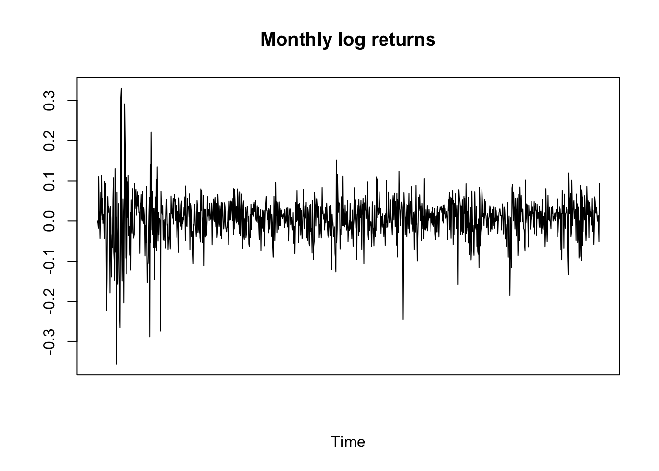
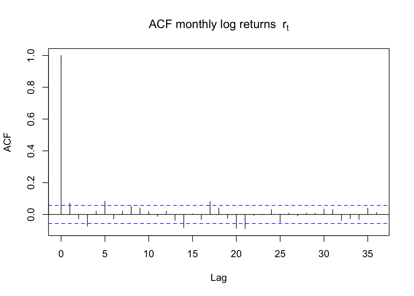
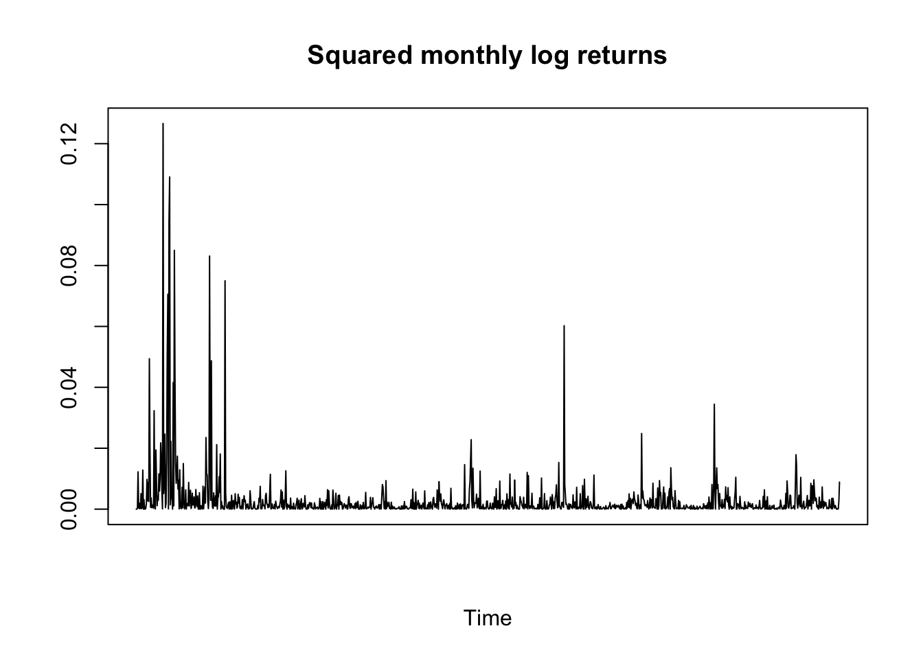
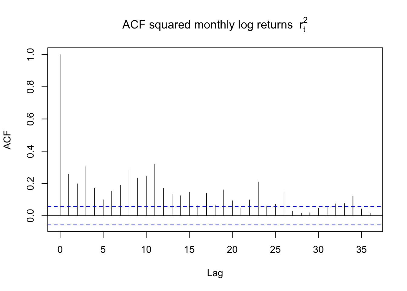
First we look at the S&P500 monthly log returns. At first, using ACF, we only see marginally significant or non-significant ACF for the log return, but the ACF for the squared log return are all significant for at least the first 20 lags, indicating non-linear serial dependence.

# Get S&P500 monthly log return
getSymbols("^GSPC", src = "yahoo", from = "1926-01-01")
price <- Cl(GSPC)
ret <- monthlyReturn(price, type = "log")

Figure 5.1

adf.test(ret) # test whether the return is stationary

    Augmented Dickey-Fuller Test

data:  ret
Dickey-Fuller = -9.3652, Lag order = 10, p-value = 0.01
alternative hypothesis: stationary

# plot margin settings
op <- par(
  mfrow = c(2,2),
  mar = c(4.5,4.5,3,1.5),
  oma = c(0.5,0.5,0.5,0.5),
  mgp = c(2.5,0.8,0),
  cex.main = 1.15,
  cex.axis = 0.9
)

par(op)

# plot the time series and the corresponding ACF for 
plot.ts(ret, main = "Monthly log returns", xlab = "Time", ylab = "", xaxt = "n")

acf(ret, lag.max = 36, main = expression("ACF monthly log returns " ~ r[t]))

plot.ts(ret^2, main = "Squared monthly log returns",
        xlab = "Time", ylab = "", xaxt = "n")

acf(ret^2, lag.max = 36, 
    main = expression("ACF squared monthly log returns " ~ r[t]^2))

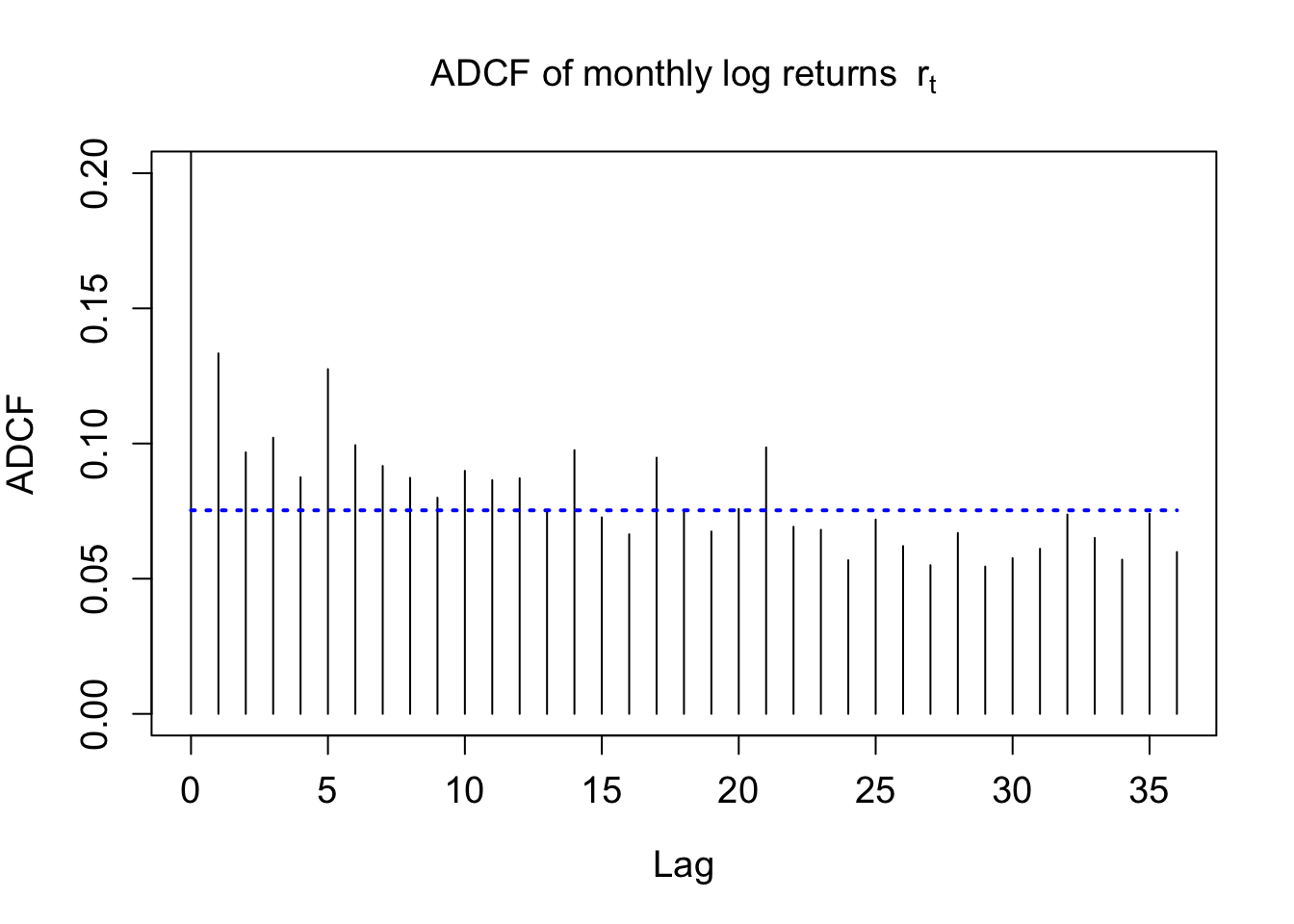
When we look at the ADCF, we detect the non-linear serial dependence with the monthly log returns.

Figure 5.2

# plot the auto-distance correlation of the S&P500 monthly log returns
dCovTS::ADCFplot(ret, ylim = c(0,0.2), MaxLag = 36, 
                 main = expression("ADCF of monthly log returns " ~ r[t]))

$ADCF
   lag 0     lag 1      lag 2     lag 3    lag 4     lag 5      lag 6
       1 0.1333414 0.09672366 0.1021607 0.087527 0.1275205 0.09939398
        lag 7      lag 8      lag 9     lag 10     lag 11     lag 12     lag 13
   0.09167906 0.08730814 0.07997258 0.08990142 0.08644292 0.08716247 0.07461983
       lag 14     lag 15     lag 16     lag 17     lag 18     lag 19     lag 20
   0.09754412 0.07267973 0.06642182 0.09477027 0.07488762 0.06745874 0.07579659
       lag 21     lag 22     lag 23    lag 24     lag 25     lag 26    lag 27
   0.09858145 0.06922814 0.06809059 0.0568206 0.07188184 0.06206972 0.0550036
       lag 28     lag 29    lag 30     lag 31     lag 32     lag 33     lag 34
   0.06690771 0.05448784 0.0576028 0.06106862 0.07373548 0.06508954 0.05704633
       lag 35     lag 36
   0.07399227 0.05987922

$bootMethod
[1] "Wild Bootstrap"

$critical.values
[1] 0.07529309

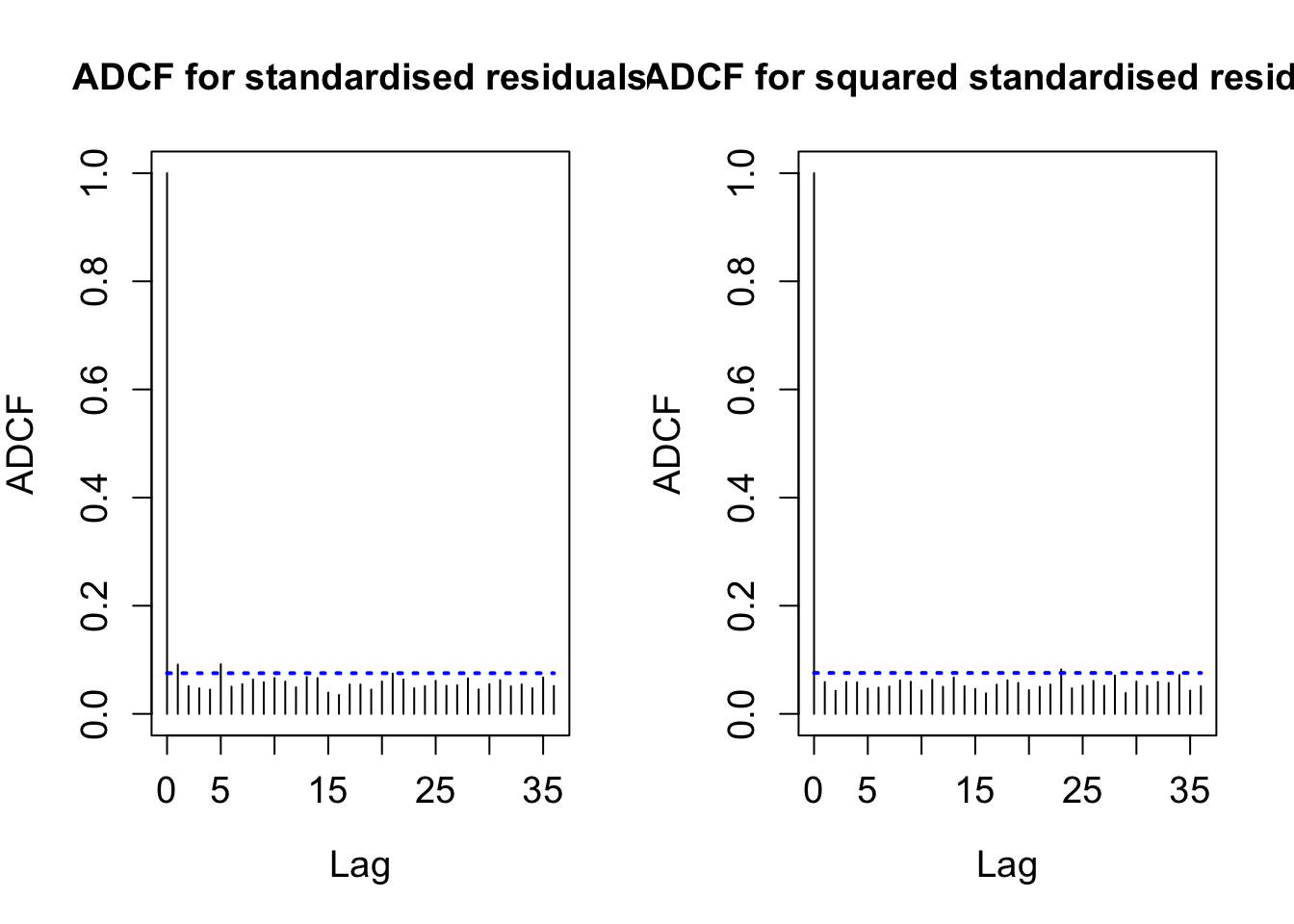
Next, we fit a GARCH(1,1) model to the S&P500 monthly log return and check the ADCF for the (squared) standardised residuals.

Figure 5.3

# GARCH(1,1), which is a benchmark model in  Awartani and Corradi (2005)

# standard GARCH
garch11 <- rugarch::ugarchspec(
  variance.model = list(model = "sGARCH", garchOrder = c(1, 1)),
  mean.model     = list(armaOrder = c(0, 0), include.mean = TRUE),
  distribution.model = "std"
)

fit_garch11 <- ugarchfit(
  spec = garch11,
  data = ret,
  solver = "hybrid",
  fit.control = list(scale = 1)
)

show(fit_garch11)

*---------------------------------*
*          GARCH Model Fit        *
*---------------------------------*

Conditional Variance Dynamics   
-----------------------------------
GARCH Model : sGARCH(1,1)
Mean Model  : ARFIMA(0,0,0)
Distribution    : std 

Optimal Parameters
------------------------------------
        Estimate  Std. Error  t value Pr(>|t|)
mu      0.008711    0.001141   7.6353 0.000000
omega   0.000099    0.000032   3.0809 0.002064
alpha1  0.133983    0.026793   5.0008 0.000001
beta1   0.830352    0.028766  28.8655 0.000000
shape   6.650187    1.209102   5.5001 0.000000

Robust Standard Errors:
        Estimate  Std. Error  t value Pr(>|t|)
mu      0.008711    0.001210   7.1995 0.000000
omega   0.000099    0.000029   3.3679 0.000758
alpha1  0.133983    0.027647   4.8462 0.000001
beta1   0.830352    0.024605  33.7476 0.000000
shape   6.650187    1.326516   5.0133 0.000001

LogLikelihood : 1994.83 

Information Criteria
------------------------------------
                    
Akaike       -3.3697
Bayes        -3.3483
Shibata      -3.3698
Hannan-Quinn -3.3616

Weighted Ljung-Box Test on Standardized Residuals
------------------------------------
                        statistic p-value
Lag[1]                     0.2927  0.5885
Lag[2*(p+q)+(p+q)-1][2]    0.3646  0.7608
Lag[4*(p+q)+(p+q)-1][5]    2.3225  0.5444
d.o.f=0
H0 : No serial correlation

Weighted Ljung-Box Test on Standardized Squared Residuals
------------------------------------
                        statistic p-value
Lag[1]                    0.03287  0.8561
Lag[2*(p+q)+(p+q)-1][5]   0.67546  0.9276
Lag[4*(p+q)+(p+q)-1][9]   1.65623  0.9418
d.o.f=2

Weighted ARCH LM Tests
------------------------------------
            Statistic Shape Scale P-Value
ARCH Lag[3]  0.008204 0.500 2.000  0.9278
ARCH Lag[5]  0.546802 1.440 1.667  0.8697
ARCH Lag[7]  1.133047 2.315 1.543  0.8910

Nyblom stability test
------------------------------------
Joint Statistic:  0.7661
Individual Statistics:              
mu     0.11483
omega  0.20241
alpha1 0.21353
beta1  0.30343
shape  0.04336

Asymptotic Critical Values (10% 5% 1%)
Joint Statistic:         1.28 1.47 1.88
Individual Statistic:    0.35 0.47 0.75

Sign Bias Test
------------------------------------
                   t-value      prob sig
Sign Bias           3.0194 0.0025874 ***
Negative Sign Bias  0.6599 0.5094621    
Positive Sign Bias  0.9641 0.3352130    
Joint Effect       20.9719 0.0001067 ***


Adjusted Pearson Goodness-of-Fit Test:
------------------------------------
  group statistic p-value(g-1)
1    20     37.34     0.007192
2    30     51.39     0.006374
3    40     61.37     0.012611
4    50     78.40     0.004822


Elapsed time : 0.02996707 

# standardized residuals
z11 <- residuals(fit_garch11, standardize = TRUE)

par(mfrow = c(1,2))
# ADCF diagnostics
dCovTS::ADCFplot(as.numeric(z11), MaxLag = 36, 
                 main = "ADCF for standardised residuals")

$ADCF
   lag 0      lag 1      lag 2      lag 3      lag 4      lag 5      lag 6
       1 0.09130349 0.05126329 0.04723894 0.04497129 0.09181725 0.05043437
        lag 7      lag 8     lag 9     lag 10     lag 11     lag 12     lag 13
   0.05511606 0.06356595 0.0585392 0.06635308 0.05984786 0.04930025 0.06807925
       lag 14     lag 15     lag 16    lag 17     lag 18     lag 19     lag 20
   0.06639491 0.03933914 0.03500954 0.0545124 0.05432607 0.04495306 0.05996097
       lag 21     lag 22     lag 23     lag 24    lag 25     lag 26     lag 27
   0.07448543 0.06383396 0.04746587 0.05154378 0.0612634 0.05210884 0.05274254
       lag 28     lag 29     lag 30     lag 31     lag 32     lag 33     lag 34
   0.06581093 0.04523578 0.05490884 0.06240159 0.05093188 0.05446399 0.04743271
       lag 35     lag 36
   0.06726309 0.05162997

$bootMethod
[1] "Wild Bootstrap"

$critical.values
[1] 0.07531128

dCovTS::ADCFplot(as.numeric(z11)^2, MaxLag = 36,
                 main = "ADCF for squared standardised residuals")

$ADCF
   lag 0      lag 1      lag 2      lag 3      lag 4      lag 5      lag 6
       1 0.05877387 0.04264124 0.05897181 0.05825753 0.04688869 0.04847001
       lag 7     lag 8      lag 9     lag 10    lag 11     lag 12     lag 13
   0.0506155 0.0619125 0.05943634 0.04340409 0.0631634 0.05024146 0.06708857
       lag 14     lag 15     lag 16   lag 17     lag 18     lag 19     lag 20
   0.05117213 0.04623772 0.03798764 0.054188 0.06208224 0.05727565 0.04390653
       lag 21     lag 22     lag 23     lag 24    lag 25     lag 26     lag 27
   0.05008773 0.05422609 0.08223865 0.04740783 0.0521891 0.06106012 0.05211128
      lag 28     lag 29     lag 30     lag 31     lag 32     lag 33     lag 34
   0.0710109 0.03852897 0.05976105 0.05171487 0.05908553 0.05711225 0.07200846
       lag 35     lag 36
   0.04307033 0.05125998

$bootMethod
[1] "Wild Bootstrap"

$critical.values
[1] 0.07574472

Los Angeles County mortality data

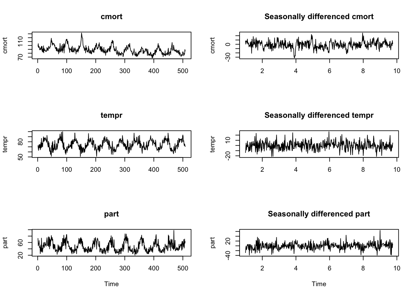
Here Shumway et al. (1988) collected weekly data on cardiovascular mortality (cmort), temperature (tempr), and pollutant particulates (part) for Los Angeles County over the period 1970–1979.

Figure 5.4

# read data
data(MortTempPart)

x <- MortTempPart[, c("cmort", "tempr", "part")]
x <- as.matrix(x)

cmort_ts <- ts(MortTempPart$cmort) 
tempr_ts <- ts(MortTempPart$tempr) 
part_ts <- ts(MortTempPart$part) 

# seasonal difference at lag 52
x_seas <- diff(x, lag = 52)
colnames(x_seas) <- c("cmort", "tempr", "part")

cmort_seas <- ts(x_seas[, "cmort"], frequency = 52)
tempr_seas <- ts(x_seas[, "tempr"], frequency = 52)
part_seas  <- ts(x_seas[, "part"],  frequency = 52)

# check stationarity for each of the time series
adf.test(cmort_ts)

Warning in adf.test(cmort_ts): p-value smaller than printed p-value

    Augmented Dickey-Fuller Test

data:  cmort_ts
Dickey-Fuller = -5.4125, Lag order = 7, p-value = 0.01
alternative hypothesis: stationary

adf.test(tempr_ts)

Warning in adf.test(tempr_ts): p-value smaller than printed p-value

    Augmented Dickey-Fuller Test

data:  tempr_ts
Dickey-Fuller = -4.4572, Lag order = 7, p-value = 0.01
alternative hypothesis: stationary

adf.test(part_ts)

Warning in adf.test(part_ts): p-value smaller than printed p-value

    Augmented Dickey-Fuller Test

data:  part_ts
Dickey-Fuller = -4.493, Lag order = 7, p-value = 0.01
alternative hypothesis: stationary

# check stationarity again
adf.test(cmort_seas, k = 20)

Warning in adf.test(cmort_seas, k = 20): p-value smaller than printed p-value

    Augmented Dickey-Fuller Test

data:  cmort_seas
Dickey-Fuller = -4.0986, Lag order = 20, p-value = 0.01
alternative hypothesis: stationary

adf.test(tempr_seas, k = 20)

Warning in adf.test(tempr_seas, k = 20): p-value smaller than printed p-value

    Augmented Dickey-Fuller Test

data:  tempr_seas
Dickey-Fuller = -4.1335, Lag order = 20, p-value = 0.01
alternative hypothesis: stationary

adf.test(part_seas, k = 20)

Warning in adf.test(part_seas, k = 20): p-value smaller than printed p-value

    Augmented Dickey-Fuller Test

data:  part_seas
Dickey-Fuller = -4.6327, Lag order = 20, p-value = 0.01
alternative hypothesis: stationary

# png("LAmort_ts.png", width = 6000, height = 5000, res = 800)
# plot the three time series

par(mfrow = c(3,2))
plot(MortTempPart$cmort, type = "l",
     main = "cmort",
     xlab = "", ylab = "cmort")

plot(cmort_seas, type = "l", 
     main = "Seasonally differenced cmort", 
     xlab = "", ylab = "cmort")

plot(MortTempPart$tempr, type = "l",
     main = "tempr",
     xlab = "", ylab = "tempr")

plot(tempr_seas, type = "l", 
     main = "Seasonally differenced tempr", 
     xlab = "", ylab = "tempr")

plot(MortTempPart$part, type = "l",
     main = "part",
     xlab = "Time", ylab = "part")

plot(part_seas,  type = "l", 
     main = "Seasonally differenced part", 
     xlab = "Time", ylab = "part")

# dev.off()

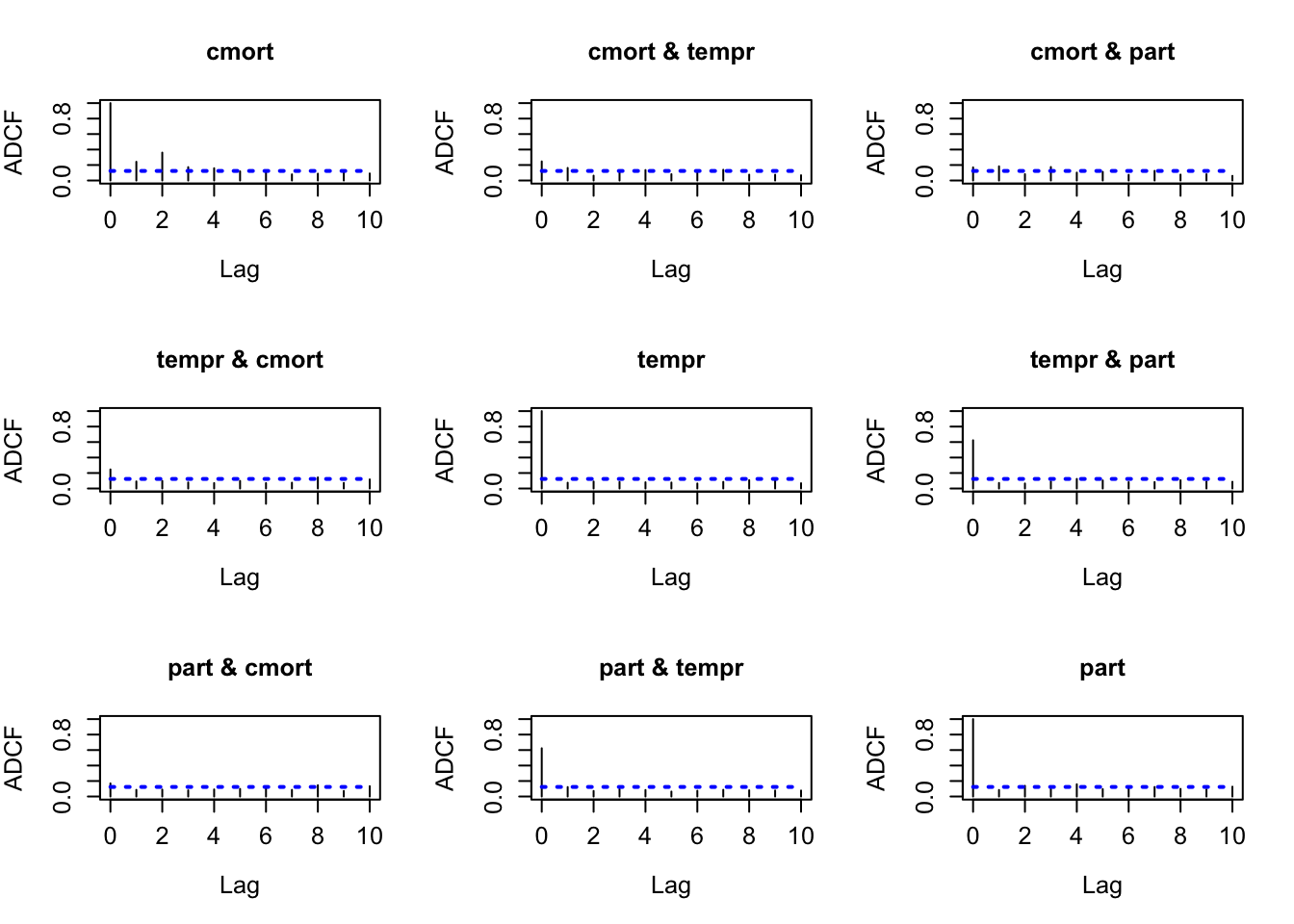
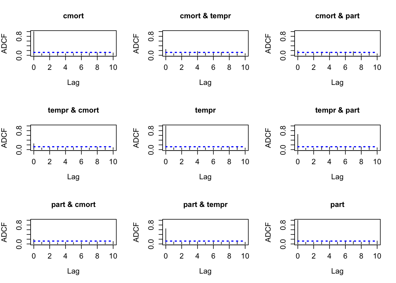
First we look at the partial ADCF and check thee lagged cross-dependence between different variables. Here we can see many of the partial ADCF are significant across different lags for each pair of the variables, motivating the use of a dynamic multivariate model.

Figure 5.5

png("mADCF_LA.png", width = 2000, height = 1600, res = 180)
mADCFplot(MortTempPart, MaxLag = 10)

$matrices
, , 1

          [,1]      [,2]      [,3]
[1,] 1.0000000 0.4538906 0.4165458
[2,] 0.4538906 1.0000000 0.1301921
[3,] 0.4165458 0.1301921 1.0000000

, , 2

          [,1]      [,2]      [,3]
[1,] 0.7011635 0.5486978 0.3615416
[2,] 0.5375026 0.6144839 0.3160165
[3,] 0.2900541 0.2477071 0.5616426

, , 3

          [,1]      [,2]      [,3]
[1,] 0.7282611 0.4805712 0.4382379
[2,] 0.4862995 0.6430712 0.3408957
[3,] 0.2535021 0.1606381 0.6062865

, , 4

          [,1]      [,2]      [,3]
[1,] 0.6294432 0.4950091 0.4162302
[2,] 0.4971926 0.5619063 0.4030866
[3,] 0.2045779 0.1402532 0.5559350

, , 5

          [,1]      [,2]      [,3]
[1,] 0.6241965 0.3816404 0.5125657
[2,] 0.4592815 0.5622770 0.4025673
[3,] 0.1483221 0.1117275 0.5345251

, , 6

           [,1]      [,2]      [,3]
[1,] 0.57250609 0.3993593 0.4852030
[2,] 0.46434222 0.5021900 0.4934183
[3,] 0.09585386 0.1108203 0.4551501

, , 7

           [,1]      [,2]      [,3]
[1,] 0.52876261 0.3434436 0.5186631
[2,] 0.44205766 0.4454101 0.4790730
[3,] 0.06482663 0.1299317 0.4561826

, , 8

           [,1]      [,2]      [,3]
[1,] 0.49366961 0.2732300 0.5416107
[2,] 0.41128076 0.4124295 0.5082240
[3,] 0.08679549 0.1731081 0.3767944

, , 9

          [,1]      [,2]      [,3]
[1,] 0.4298788 0.2263228 0.5370600
[2,] 0.3891477 0.3635864 0.4932065
[3,] 0.1398711 0.2460081 0.3172543

, , 10

          [,1]      [,2]      [,3]
[1,] 0.4037443 0.1809716 0.4934697
[2,] 0.3399371 0.3064618 0.5061619
[3,] 0.1595501 0.2948185 0.2431079

, , 11

          [,1]      [,2]      [,3]
[1,] 0.3476185 0.1503438 0.4884442
[2,] 0.3090137 0.2212398 0.4834152
[3,] 0.2152796 0.3345741 0.2122764


$bootMethod
[1] "Wild Bootstrap"

$critical.value
[1] 0.1180574

dev.off()

quartz_off_screen 
                2 

x_seas_ts <- ts(
  cbind(cmort = cmort_seas,
        tempr = tempr_seas,
        part  = part_seas),
  frequency = 52
)
# png("mADCF_LA_diff.png", width = 2000, height = 1600, res = 180)
mADCFplot(x_seas_ts, MaxLag = 10)

$matrices
, , 1

          [,1]      [,2]      [,3]
[1,] 1.0000000 0.2465233 0.1693315
[2,] 0.2465233 1.0000000 0.6233087
[3,] 0.1693315 0.6233087 1.0000000

, , 2

           [,1]       [,2]       [,3]
[1,] 0.24176663 0.16230028 0.18309403
[2,] 0.09162115 0.07454006 0.07140625
[3,] 0.08589254 0.12179757 0.08422251

, , 3

           [,1]       [,2]       [,3]
[1,] 0.36043693 0.06252492 0.08180086
[2,] 0.09798584 0.09029595 0.06507049
[3,] 0.08957948 0.07168032 0.13814648

, , 4

           [,1]       [,2]       [,3]
[1,] 0.17245327 0.12069083 0.17429476
[2,] 0.07790478 0.08384162 0.09105514
[3,] 0.07987314 0.09428095 0.09527002

, , 5

           [,1]       [,2]      [,3]
[1,] 0.15838425 0.13500097 0.1020670
[2,] 0.07016221 0.08023236 0.1238285
[3,] 0.09131852 0.08387354 0.1580887

, , 6

           [,1]       [,2]       [,3]
[1,] 0.11818126 0.08148086 0.11178527
[2,] 0.09812425 0.07729116 0.10428837
[3,] 0.09804394 0.06391040 0.09548868

, , 7

           [,1]       [,2]       [,3]
[1,] 0.10664405 0.09980273 0.07320061
[2,] 0.06975426 0.06509267 0.08192176
[3,] 0.11130541 0.07437038 0.11546785

, , 8

           [,1]       [,2]       [,3]
[1,] 0.07925822 0.13855139 0.12506973
[2,] 0.07509925 0.08597505 0.08344496
[3,] 0.08605257 0.08677822 0.12324069

, , 9

           [,1]       [,2]       [,3]
[1,] 0.08817903 0.07548946 0.07628336
[2,] 0.14344446 0.10745907 0.10699561
[3,] 0.14595343 0.08040806 0.09868926

, , 10

           [,1]       [,2]       [,3]
[1,] 0.10459255 0.07469886 0.08107945
[2,] 0.07207610 0.11556270 0.08981952
[3,] 0.07190897 0.07750890 0.09230887

, , 11

           [,1]       [,2]       [,3]
[1,] 0.09119371 0.06797147 0.06014913
[2,] 0.11758988 0.06839344 0.08682843
[3,] 0.13348982 0.07731398 0.12701236


$bootMethod
[1] "Wild Bootstrap"

$critical.value
[1] 0.1235711

# dev.off()

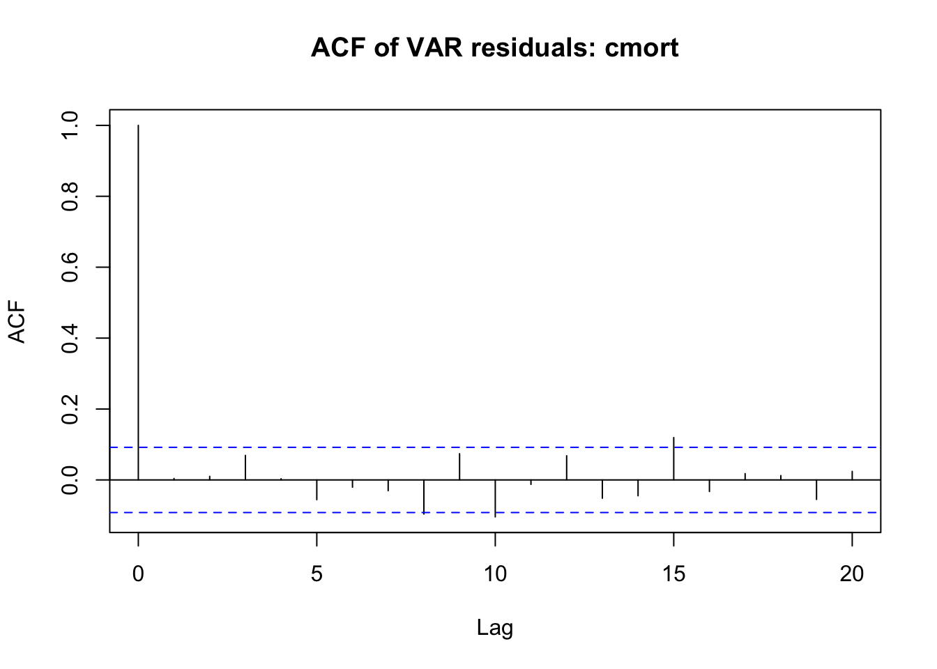
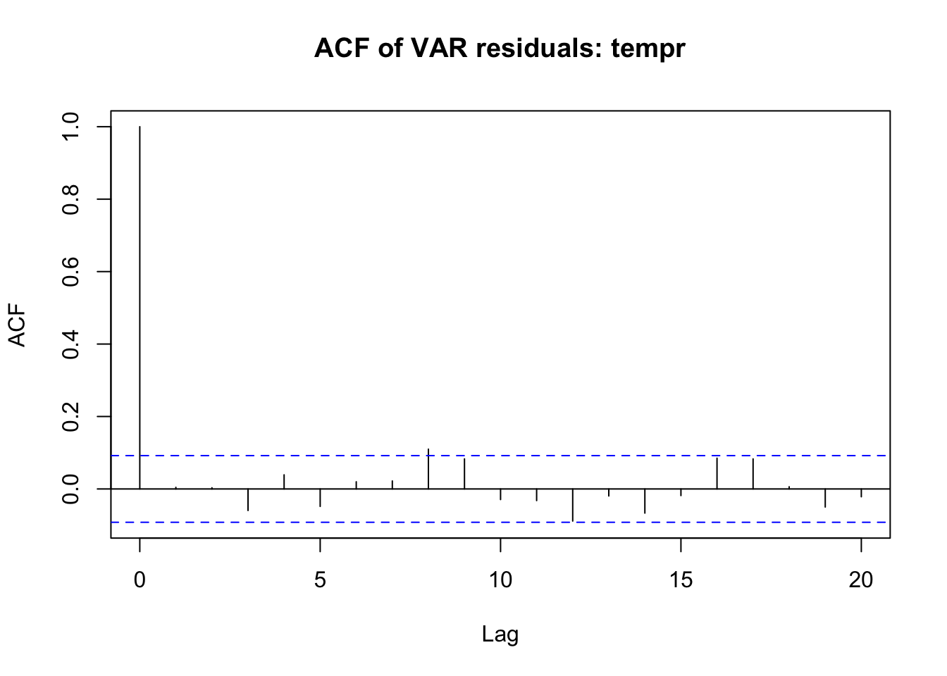
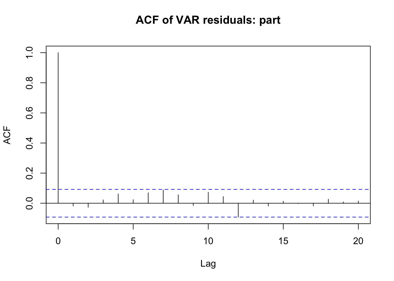
Now we fit a VAR(2) model to the three time series and verify the fitness by checking the partial ADCF of the residuals. The (partial) ADCF is insignificant for most lags both within and across pairs of series, suggesting a good fit.

Figure 5.6

VARselect(x_seas, lag.max = 10, type = "const")$selection

AIC(n)  HQ(n)  SC(n) FPE(n) 
     5      2      2      5 

# fit VAR with p=2
fit_var <- VAR(x_seas_ts, p = 2, type = "const")
summary(fit_var)

VAR Estimation Results:
========================= 
Endogenous variables: cmort, tempr, part 
Deterministic variables: const 
Sample size: 454 
Log Likelihood: -4800.476 
Roots of the characteristic polynomial:
0.7447 0.4728 0.4623 0.3738 0.2322 0.1741
Call:
VAR(y = x_seas_ts, p = 2, type = "const")


Estimation results for equation cmort: 
====================================== 
cmort = cmort.l1 + tempr.l1 + part.l1 + cmort.l2 + tempr.l2 + part.l2 + const 

          Estimate Std. Error t value Pr(>|t|)    
cmort.l1  0.259392   0.046550   5.572 4.35e-08 ***
tempr.l1 -0.135324   0.058697  -2.305   0.0216 *  
part.l1  -0.078177   0.033118  -2.361   0.0187 *  
cmort.l2  0.321994   0.045660   7.052 6.74e-12 ***
tempr.l2  0.006543   0.058822   0.111   0.9115    
part.l2  -0.026449   0.033016  -0.801   0.4235    
const    -0.547469   0.349815  -1.565   0.1183    
---
Signif. codes:  0 '***' 0.001 '**' 0.01 '*' 0.05 '.' 0.1 ' ' 1


Residual standard error: 7.329 on 447 degrees of freedom
Multiple R-Squared: 0.2661, Adjusted R-squared: 0.2563 
F-statistic: 27.02 on 6 and 447 DF,  p-value: < 2.2e-16 


Estimation results for equation tempr: 
====================================== 
tempr = cmort.l1 + tempr.l1 + part.l1 + cmort.l2 + tempr.l2 + part.l2 + const 

         Estimate Std. Error t value Pr(>|t|)
cmort.l1 -0.06893    0.05063  -1.361    0.174
tempr.l1  0.04240    0.06385   0.664    0.507
part.l1  -0.02173    0.03602  -0.603    0.547
cmort.l2  0.01465    0.04967   0.295    0.768
tempr.l2  0.07881    0.06398   1.232    0.219
part.l2  -0.03745    0.03591  -1.043    0.298
const    -0.15394    0.38051  -0.405    0.686


Residual standard error: 7.972 on 447 degrees of freedom
Multiple R-Squared: 0.01007,    Adjusted R-squared: -0.003222 
F-statistic: 0.7575 on 6 and 447 DF,  p-value: 0.6037 


Estimation results for equation part: 
===================================== 
part = cmort.l1 + tempr.l1 + part.l1 + cmort.l2 + tempr.l2 + part.l2 + const 

           Estimate Std. Error t value Pr(>|t|)   
cmort.l1  0.0220204  0.0864014   0.255  0.79895   
tempr.l1 -0.1783699  0.1089461  -1.637  0.10229   
part.l1   0.0004458  0.0614709   0.007  0.99422   
cmort.l2 -0.1934024  0.0847484  -2.282  0.02295 * 
tempr.l2 -0.1077074  0.1091789  -0.987  0.32441   
part.l2   0.1611094  0.0612813   2.629  0.00886 **
const    -0.7231947  0.6492886  -1.114  0.26595   
---
Signif. codes:  0 '***' 0.001 '**' 0.01 '*' 0.05 '.' 0.1 ' ' 1


Residual standard error: 13.6 on 447 degrees of freedom
Multiple R-Squared: 0.03674,    Adjusted R-squared: 0.02381 
F-statistic: 2.841 on 6 and 447 DF,  p-value: 0.01002 



Covariance matrix of residuals:
      cmort tempr   part
cmort 53.71 16.69  21.35
tempr 16.69 63.55  72.38
part  21.35 72.38 185.05

Correlation matrix of residuals:
       cmort  tempr   part
cmort 1.0000 0.2856 0.2142
tempr 0.2856 1.0000 0.6674
part  0.2142 0.6674 1.0000

E <- residuals(fit_var)

op <- par(mfrow = c(3, 1), mar = c(4, 4, 2, 1))
par(op)

# check ACF of the residuals
acf(E[, "cmort"], lag.max = 20, main = "ACF of VAR residuals: cmort")

acf(E[, "tempr"], lag.max = 20, main = "ACF of VAR residuals: tempr")

acf(E[, "part"],  lag.max = 20, main = "ACF of VAR residuals: part")

# png("mADCF_LA_VAR_res.png", width = 2000, height = 1600, res = 180)
mADCFplot(E, MaxLag = 10)

$matrices
, , 1

          [,1]      [,2]      [,3]
[1,] 1.0000000 0.2511320 0.1959196
[2,] 0.2511320 1.0000000 0.6438999
[3,] 0.1959196 0.6438999 1.0000000

, , 2

           [,1]       [,2]       [,3]
[1,] 0.06698650 0.06650183 0.06505325
[2,] 0.07150791 0.07852114 0.05986357
[3,] 0.07569272 0.08577160 0.07198033

, , 3

           [,1]       [,2]       [,3]
[1,] 0.07691076 0.07965485 0.08774187
[2,] 0.09646864 0.07132115 0.06791220
[3,] 0.08800707 0.07766143 0.07019281

, , 4

           [,1]       [,2]       [,3]
[1,] 0.08372035 0.07304465 0.09367255
[2,] 0.07391701 0.08186113 0.09263560
[3,] 0.05128032 0.08700100 0.07008528

, , 5

           [,1]       [,2]      [,3]
[1,] 0.06744168 0.16183217 0.1284962
[2,] 0.08078728 0.07975176 0.1069115
[3,] 0.07443823 0.09129686 0.1205908

, , 6

           [,1]       [,2]       [,3]
[1,] 0.07776394 0.08590217 0.09528166
[2,] 0.08355052 0.08036080 0.09703343
[3,] 0.05998376 0.06326831 0.07524575

, , 7

           [,1]       [,2]       [,3]
[1,] 0.06846701 0.08148717 0.08426613
[2,] 0.07345406 0.06184579 0.08372921
[3,] 0.06679096 0.07692052 0.08960361

, , 8

           [,1]       [,2]       [,3]
[1,] 0.08857210 0.12422649 0.15542555
[2,] 0.06982066 0.08133445 0.08635416
[3,] 0.06890333 0.07566945 0.10822032

, , 9

           [,1]       [,2]       [,3]
[1,] 0.10789471 0.06750178 0.06861208
[2,] 0.10736955 0.11429887 0.11126405
[3,] 0.08977336 0.09143449 0.07852424

, , 10

           [,1]       [,2]       [,3]
[1,] 0.09161540 0.07184912 0.08563192
[2,] 0.07528669 0.11099173 0.08147873
[3,] 0.06512839 0.09217182 0.08038913

, , 11

           [,1]       [,2]       [,3]
[1,] 0.10444237 0.07145906 0.06442142
[2,] 0.08790636 0.07111244 0.08095578
[3,] 0.10829264 0.07439416 0.12663960


$bootMethod
[1] "Wild Bootstrap"

$critical.value
[1] 0.1212314

# dev.off()

References

Avanzi, Benjamin, Guillaume Boglioni Beaulieu, Pierre Lafaye de Micheaux, Frédéric Ouimet, and Bernard Wong. 2021. “A Counterexample to the Existence of a General Central Limit Theorem for Pairwise Independent Identically Distributed Random Variables.” Journal of Mathematical Analysis and Applications 499 (1): 124982.

Beaulieu, Guillaume Boglioni, Pierre Lafaye de Micheaux, and Frédéric Ouimet. 2021. “Counterexamples to the Classical Central Limit Theorem for Triplewise Independent Random Variables Having a Common Arbitrary Margin.” arXiv Preprint arXiv:2104.02292.

Central Intelligence Agency. 2020. The World Factbook.

Shumway, RH, AS Azari, and Y Pawitan. 1988. “Modeling Mortality Fluctuations in Los Angeles as Functions of Pollution and Weather Effects.” Environmental Research 45 (2): 224–41.